Cowboy Programming Game Development and General Hacking by the Old West

April 1, 2008

Practical Fluid Mechanics

Filed under: Game Development,Inner Product — Mick West @ 1:57 pm

(This article originally appeared in two parts in Game Developer Magazine, March and April, 2007) Fluid effects such as rising smoke and turbulent water flow are everywhere in nature, but are seldom implemented convincingly in computer games. The simulation of fluids (which covers both liquids and gasses) is computationally very expensive. It is also mentally very expensive, with even introductory papers on the subject relying on the reader having math skills at least at the undergraduate calculus level.

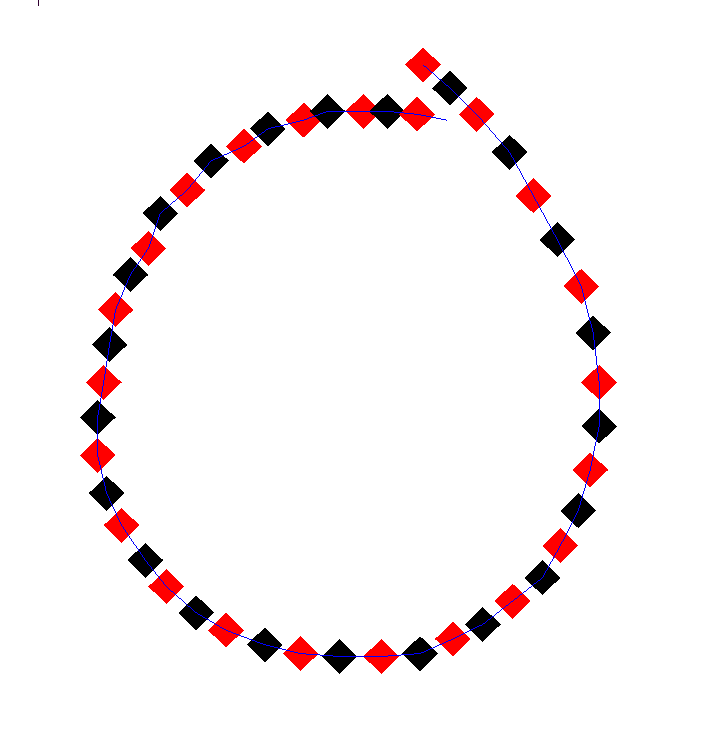
In this article I will attempt to address both these problems from the perspective of a game programmer not necessarily conversant with vector calculus. I’ll explain how certain fluid effects work without using advanced equations and without too much new terminology. I shall also describe one way of implementing the simulation of fluids in an efficient manner without the expensive iterative diffusion and projection steps found in other implementations. A working demonstration with source accompanies this article and can be downloaded from here, example output from this can be seen in figure 1.

Figure 1 - Sample Output

GRIDS OR PARTICLES?

There are several ways of simulating the motion of fluids. These generally divide into two common types of methods: grids methods and particle methods. In grid methods, the fluid is represented by dividing up the space a fluid might occupy into individual cells, and storing how much of the fluid is in each cell. In particle methods the fluid is modeled as a large number of particles that each move around and react to collision with the environment and interacting with nearby particles. Here I’m going to concentrate on simulating fluids with grids.

It is simplest to discuss the grid methods with respect to a regular two-dimensional grid, although the techniques apply equally well to three dimensions. At the simplest level, to simulate fluid in the space covered by a grid you need two grids, one to store the density of liquid or gas at each point, and another to store the velocity of the fluid. Figure 2 shows a representation of this, with each point having a velocity vector, and also containing a density value (not shown). The actual implementation of these grids in C/C++ is most efficiently done as one dimensional arrays. The amount of fluid in each cell is represented as a float. The velocity grid (also referred to as a velocity field, or vector field) could be represented as an array of 2D vectors, but for coding simplicity it is best represented as two separate arrays of floats, one for x and one for y.

In addition to these two grids we can have any number of other matching grids that store various attributes. Again each will be stored as matching array of floats, and can store things such as the temperature of the fluid at each point, or the color of the fluid (whereby you can mix multiple fluids together). You can also store more esoteric quantities such as humidity, for if you were simulating steam or cloud formation.

ADVECTION

The fundamental operation in grid based fluid dynamics is advection. Advection is basically moving things around on the grid, but more specifically it’s moving the quantities stored in one array by the movement vectors stored in the velocity arrays. It’s quite simple to understand what is going on here if you think of each point on the grid as being an individual particle, with some attribute (the density) and a velocity.

You are probably familiar with the process of moving a particle by adding the velocity vector to the position vector. On the grid, however, the possible positions are fixed, so all we can do is move (advect) the quantity (the density) from one grid point to another. In addition to advecting the density value, we also need to advect all the other quantities associated with the point. This would obviously include additional attributes such as temperature and color, but also includes the velocity of the point itself. The process of moving a velocity field over itself is referred to as self-advection.

The grid does not represent a series of discreet quantities, density or otherwise, it actually represents (inaccurately) a smooth surface, with the grid points just being sampled points on that surface. Think of the points as being X,Y vertices of a 3D surface, with the density field being the Z height. Thus you can pick any X and Y position on the mesh, and find the Z value at that point by interpolating between the closest four points. Similarly while advecting a value across the grid the destination point will not fall directly on a grid point, and you will have to interpolate your value into the four grid points closest to the target position.

In figure 3, the point at P has a velocity V, which, after a time step of dt, will put it in position P’ = P + dt*V. This point falls between the points A, B, C and D, and so a bit of P has to go into each of them. Generally dt*V will be significantly smaller than the width of a cell, so one of the points A,B,C or D will be P itself. Advecting the entire grid like this sufferers from various inaccuracies, particularly that quantities dissipate when moving in a non-axis-axis-aligned direction. This inaccuracy can actually be turned to our advantage.

STAM’S ADVECTION

Programmers looking into grid based fluid dynamics for the first time will most often come across the work of Jos Stam and Ron Fedkiw, particularly Stam’s paper “Real-Time Fluid Dynamics for Games“, presented at the 2003 Game Developer Conference. In this paper Stam presents a very short implementation of a grid based fluid simulator. In particular he describes implementing the advection step using what he terms a “linear backtrace”, which simply means instead of moving the point forward in space, we invert the velocity and find the source point in the opposite direction, essentially back in time. We then take the interpolated density value from that source (which, again, will lay between four actual grid points), and then move this value into the point P. See figure 4.

Stam’s approach produces visually pleasing results, yet suffers from a number of problems. Firstly the specific collection of techniques discussed may be covered by U.S. patent #6,266,071, although as Stam notes, the approach of backtracing dates back to 1952. Check with your lawyer if this is a concern to you. On a more practical note the advection alone as described by Stam simply does not work accurately unless the velocity field is smooth in a way termed mass conserving, or incompressible.

Consider the case of a vector field where all the velocities are zero except for one. In this situation the velocity cannot move (advect) forward through the field, since there is nothing ahead of it to “pull” it forward, instead the velocity simply bleeds backwards. The resultant velocity field will terminate at the original point, and any quantities moving through this field will end up there. This problem is solved by adding a step to the algorithm termed projection, which is basically smoothes out the velocity by making it incompressible, thus allowing the backtracing advection to work perfectly, and making the paths formed by the velocity be “swirly”, as would be the case in real water.

The problem with this approach is that projection is quite expensive, requiring 20 iterations over the velocity field in order to “relax” it to a usable state. Another performance problem with Stam’s approach is that there is a diffusion step, which also involves 20 iterations over a field. This is needed to allow the gas to spread out from areas of high density to areas of low density. If the diffusion step were missing, solid blocks of the fluid would remain solid as them moved over the velocity field. The diffusion is an important cosmetic step in the process.

ACCOUNTING ADVECTION

If a velocity field is not mass conserving, then this means that some points will have multiple velocity vectors from other points pointing towards them. This means that if we simply move our scalar quantities (like density) along these vectors, then there will be multiple quantities going to (or coming from) the same point, and the result will be a net loss or gain of the scalar quantity. So if the total amount of something such as the density would either fade to zero or gradually (or perhaps explosively) increase.

The usual solution to this problem is to make sure the vector field is incompressible and mass conserving. But as mentioned before, this is computationally expensive. One partial solution is to make the advection step mass conserving, regardless of if the velocity field actually is mass conserving. The basis of this solution is to always account for any movement of a quantity by subtracting in one place what is added in another. Advection uses a source and destination buffer to keep it independent of update order. In Stam’s implementation, the destination buffer is simply filled one cell at a time by combining a value from four cells in the source buffer, and placing this value into the destination buffer.

To properly account for compressible motion, we need to change this copying to accumulating, and initially make the destination buffer a copy of the source buffer, and as we move quantities from one place to another we can subtract them in the source and add them in the destination. With the forward advection in figure 3, we are moving a quantity from point P to points A,B,C and D. To account for this we simply subtract the original source value in P from the destination value in P, and then add it (interpolated appropriately), to A,B,C,D. The net change on the destination buffer is zero. With the reverse advection in figure 4, as used by Stam, the solution would initially seem to be symmetrically the same: just subtract the interpolated source values in E,F,G and H from the destination buffer, and add them to P.

While this works fine for signed quantities such as velocity, the problem here is that quantities such as density are positive values. They cannot go below zero as you cannot have a negative quantity of a liquid. Suppose that point E was one source point for two destinations P1 and P2, both of which wanted 0.8 of E. Now, if we follow our initial plan and subtract 0.8*E from E and add 0.8*E to both P1 and P2, the net effect is zero, but now the value at E is negative. If we clamp E to zero then there is a net gain of 0.6*E. If we subtract 0.8*E from the source value of E after updating P1, then when we update P2 it will only get 0.8*0.2*E, when clearly both P1 and P2 should both get equal amounts, and intuitively here it seems they should both get 0.5*E, and the resulting value in E should be zero, leading to a net zero change.

To achieve this result I first create a list that for each point records the four points that are sources for that point, and the fraction of each point they want. Simultaneously I accumulate the fractions asked of each source point. In an ideal world, this would add up to one, as the entire value is being moved somewhere (including partially back where it started). But with our compressible field the amount of the value in each point that is being moved can be greater than or less than one. If the total fraction required is greater than one, then we can simply scale all the requested fraction by this value, which means the total will be one. If less than one, then the requesting points can have the full amount requested. We should not scale in this case as it will lead to significant errors.

With the mass conservation of advection fully accounted for in both directions, it turns out that neither forward or backward linear advection alone will produce smooth results. After some experimentation I determined that applying forward advection followed by backward advection worked very well, and give a very smooth and artifact free flow of fluid over a compressible velocity field.

NOW WHAT?

So, we can now perform both forward and reverse advection in a mass-conserving manner, meaning we can move fluid around its own velocity field. But even though our velocity field does not need to be mass-conserving, we actually still want it to be, since the velocity fields of real world fluids generally are incompressible. Stam solves this problem by expensively forcing the field to be fully mass conserving after every change. This is necessary, since the reverse advection requires it. The key difference now is that since our advection step does not require the field to be mass-conserving, we are really only doing it for cosmetic purposes. To that end, any method that rapidly approaches that state over several time-steps will suit our purpose. That method, and the method of diffusion, can be found in the accompanying code, and are discussed below.

PRACTICAL FLUID DYNAMICS: PART 2

In last month’s article (above) I gave an overview of the nuts and bolts behind simple two dimensional fluid dynamics using a grid system. This month I’ll expand upon this, explaining how we can achieve a reasonable level of realism without too many expensive iterations. I’ll also continue with my goal of explaining how everything works by using no math beyond basic algebra.

50 x 50 velocity field, click to view full sizeTo recap so far: we have a velocity field which is an array of cells, each of which stores the velocity at a particular point (click example on the right). Remember this a continuous field, and we can get the velocity at any point on the field surface (or in the field volume for 3D), by interpolating between the nearest points on the field. We also have a matching field of density. The density field represents how much of the fluid or gas is in a particular grid cell. Again this a continuous field, and you can get a density value for any point in the simulated space by interpolating. I then described the process of advection, which is the moving of the values in one field (say the density field), over the velocity field.

I described both forward advection and reverse advection, where the quantities in the field are respectively pushed out of a cell, or pulled into a cell by the velocity at that cell. I noted that the advection process worked well if you perform forward advection and then follow it with reverse advection.

INCOMPRESSIBLE FIELDS

I noted that reverse advection in particular would only work if the velocity field was in a state termed incompressible. But what does this mean? Well, you might have heard that “water is incompressible”, meaning you can’t squeeze water into a smaller volume than it already occupies. Compare this with gasses such as air, where you can clearly be compressed. Picture, for example, a diver’s air tank. The tank contains a lot more air than the volume occupied by the tank. But if you were to take that tank, and fill it with water, and then somehow push in another pint of water, then the tank would explode.

Water, in fact, is actually compressible, very slightly, since it’s physically impossible to have a truly incompressible form of matter. The incompressibility of a material is measured by a metric called a “bulk modulus”, For air this is about 142,000 whereas for water, it’s 2,200,000,000 or approximately 15,000 times as much. By comparison, the least compressible substance known to humankind, aggregated diamond nanorods, are just 500 times more incompressible than water.

So for most practical purposes, you can imagine water as being incompressible. So, with water being considered incompressible, then when considering a solid volume of water, there can not be more water in one cell than in another. So, if we start out with an equal amount of water in each cell, then after moving the water along the velocity field (advecting), we can’t increase or decrease the amount of water in each cell. If this happens, then the velocity field is incompressible or mass conserving.

PRESSURE

You can think of the pressure at a particular node as being the difference in density between a cell and its neighbors. Now with water being incompressible, the pressure is going to be the same throughout the density field. If we think of a node as having a series of inputs and outputs during the advection process, then in an incompressible field, the sum of input is equal to the sum of outputs (Figure 5a). When we move the water along its incompressible velocity field, then the density at each node will remain constant, and hence the pressure will remain constant.

On the other hand, if the velocity field happens to be structured in such a way that for some cells more is going into them then is coming out, then the velocity field is compressible (Figure 5b). When the density of the fluid is advected across a compressible velocity field, then the density in individual cells will increase or decrease. If we simply keep advecting the density, then the density will eventually all be compressed into the cells of the velocity field that have a net gain of input over output.

If we were not performing accounting in our advection step (as explained last month), then there would be an overall net loss in density (the field is not mass conserving). Stepping back from our abstraction for a second, what prevents this from happening in real-life? Well, obviously if more of a fluid flows into a cell than is flowing out, then the density of that cell increases relative to its neighbors, and hence the pressure in that cell increases. High pressure in a cell creates an acceleration force on the neighboring cells, increasing their velocity away from that cell, hence increasing the outflow rate from the cell, and evening out the imbalance. As with the atmosphere, fluid flows from an area of high pressure to an area of low pressure.

APPLYING PRESSURE

Listing 1 shows the code for applying pressure. Here mp_p0 is the array that stores the density (which is equivalent to the pressure, so I actually refer to it as pressure in the code). The arrays mp_xv1 and mp_yv1 store the x and y components of the velocity field. The function Cell(x,y) returns a cell index for a given set of x and y coordinates. The loop simply iterates over all horizontal and vertical pairs of cells, finds the difference in pressure, scales it by a constant (also scaled by time) and adds it to both cells.

The logic here is slightly unintuitive, since physics programmers are used to the Newtonian principle that every action has an equal an opposite reaction, yet here when we add a force, there is no opposing force, and we don’t subtract a force from anywhere else. The reason is clear if you consider what is actually going on. We are not dealing with Newtonian mechanics. The force actual comes from the kinetic energy of the molecules of the fluid which are actually randomly traveling in all directions (assuming the fluid is above absolute zero), and the change to the velocity field actually happens evenly across the gradient between the two points, so in effect we are applying the resultant force from a pressure gradient to the area it covers, which here is two cells, and we divide it between them.

Here’s an example, just looking in the x direction, we have a flat pressure field, with one cell denser that the rest. The cell densities are 4,4,5,4,4. The gradients between the four pairs of cells is 0,-1,+1,0 Adding this to each cell (ignoring scaling), we get: 0,-1,0,+1,0. See Figure 6.

Here the cells on either side of the high pressure cell end up with a velocity pointing away from that cell. Consider now what will happen with the advection step, the reverse advection combined with forward advection will move the high pressure cell outwards, reducing the pressure, and reducing the force. The fluid moves from an area of high pressure to an area of low pressure.

Effectively this makes the velocity field tend towards being incompressible and mass conserving. If there is a region that is increasing in density, then the resultant increase in pressure will turn the velocity field away from that area, and hence decrease the density in that area. Eventually the velocity field will either become mass conserving (mass just circulating without density change), or it will stop (become zero).

Listing 1 – The pressure differential between two cells creates an identical force on both cells

for (int x = 0; x < m_w-1; x++) {
for (int y = 0; y < m_h-1; y++) {
int cell = Cell(x,y);
float force_x =  mp_p0[cell] - mp_p0[cell+1];
float force_y =  mp_p0[cell] - mp_p0[cell+m_w];
mp_xv1[cell]     +=  a * force_x;
mp_xv1[cell+1]   +=  a * force_x;
mp_yv1[cell]     +=  a * force_y;
mp_yv1[cell+m_w] +=  a * force_y;
}

INK AND SMOKE

What we are modeling here is motion within a fluid (such as air swirling around inside a room), and not the overall motion of a volume of water, (such as water sloshing around a cup. This method, as it stands, does not simulate the surface of the fluid. As such, visualizing the fluid itself is not very interesting, since a room full of air looks pretty much the same regardless of how the air is moving. Where it become interesting is when we introduce some substance into the fluid that is suspended by that fluid, and carried around by the fluid.

In water this could be silt, sand ink, or bubbles. In air, it could be dust, steam, or smoke. You can even use the velocity field techniques outlined here to move larger object such as leaves or paper in a highly realistic manner. Note it’s important that what we are talking about is a suspension of one substance in another. We are generally not so interested in simulating two fluids that do not mix (like oil and water).

Games have things that burn and explode, so smoke is a very common graphical effect. Smoke is not a gas, but a suspension of tiny particles in the air. These tiny particles are carried around by the air, and they comprise a very small percentage of the volume occupied by the air. So we do not need to be concerned about smoke displacing air.

In order to simulate smoke, we simply add another advected density field matching, where the value at each cell represents the density of smoke in that region. In the code this is referred to as “ink”. This is similar to the density of air, except the density of smoke or ink is more of a purely visual thing, and does not affect the velocity field.

HEATING THINGS UP

One final ingredient that often goes along with a fluid system like this is the heat of the fluid/gas at each location. Sources of smoke are usually hot, which heats up the air the smoke initially occupies. This causes the smoke to rise. It rises because higher temperatures mean more energy, which means the fluid molecules are moving faster, which means higher pressure, which means lower density (remember density is only proportional to pressure at constant temperature), which makes the hot air rise.

Now, that’s a complex sequence of events, but it’s initially simpler to just model the result, “hot air rises”, and have the relative temperature of a cell create a proportionate upwards force on the velocity field at that cell. We can do this trivially by adding a scaled copy of the heat field to the Y velocity field. Similarly, rather than attempt to model the effects of heat in the initial phases of a simulation, I found it easier to simply model the expected results.

So, although a flame creates heat which makes the smoke rise, more pleasing results were found by “manually” giving the volume of air around the flame an initial upwards velocity, and then letting the heat take it from there. With more complex systems such as an explosion, the fiddly physics happens in the first tenth of a second, so you can just skip over that and set up something that looks visually pleasing with our simplified physics.

FILTERING THINGS OUT

The simplistic application of forces we perform for acceleration due to pressure (Figure 2) has the tendency to introduce artifacts into the system. These typically present as unnatural looking ripples. The way these are dealt with is to smooth out the velocity and pressure fields by applying a simple diffusion filter. If you use the Stam style reverse advection with projection, then you have to use a computationally intensive filter iterating several time. But with the inherent diffusion of forward advection, combined with the accuracy of the combined forward and backwards accounted advection, we can get away with a single iteration.

It’s often difficult to see exactly what effect a change can have on a fluid system such as this. The fluid is very complex looking, and small changes to parameters often have an effect that is not immediately obvious. The ideal way to solve this problem is to set up your system so you can run two copies of the same system in parallel, with one having the modified parameters. The difference can then become obvious. Figure 7 (below) shows such an A/B comparison. The image on the left has no diffusion filtering, and the image on the right has a single pass of diffusion filtering applied every update.

FLUID IDEAS

I’ve glossed over a few other important aspects here, but details of these aspects can be found in the accompanying code. You need to pay particular attention to how you handle the cells that are at the edge of the system, as the differing number of neighbors has a significant effect. At the edges of a system you have the option of either reflecting, wrapping or zeroing values, depending on what you want. By wrapping in one direction you essentially get a tiling animated texture in that direction, which could be used as a diffusion or displacement map for the surface of a moving stream of fluid .

There is also the issue of friction. Motion in a fluid is generally quite viscous. This can be implemented as a simple friction force that applies to the velocity field. If there is no friction in the fluid it can slosh around forever, which is generally not what you want. Different viscosity setting give very different visual results. There are a very large number of variables that can be tweaked to give radically difference visual effects, even in my rather simple implementation. It’s worthwhile spending some time just playing with these values just to see what happens.

Additional resources

3D Version

This approach has also been implemented in 3D by Quentin Froemke, et al, at Intel, as part of their research into Multi Threaded programming.

http://www.gamasutra.com/view/feature/4022/sponsored_feature_multithreaded_.php

March 23, 2008

Debugging Heisenbugs

Filed under: Game Development,Inner Product — Mick West @ 4:29 pm

(This article originally appeared in Game Developer Magazine, October 2007, in a slightly different format)

A Heisenbug is a type of bug that disappears or alters its behavior when you attempt to debug it. The word “Heisenbug” is a slight misnomer, referencing Heisenberg’s uncertainty principle, which describes how, in quantum physics, it is impossible to know both where something is, and how fast it is. A related phenomenon is the “observer effect”, which says you cannot observe something without altering it – this “observer effect” is what causes the problems we call Heisenbugs.

Heisenbugs are common in game development, most frequently in lower level code. A programmer may encounter several such bugs in the course of development, and a failure to appropriately handle them can seriously derail development, as it may take many days to track down the elusive bug. This article discusses some of the causes of Heisenbugs, and gives some guidelines for avoiding them and tracking them down.

RANDOM CAUSES

The causes of Heisenbugs are as varied as the causes of regular bugs. But some factors are more likely to result in a Heisenbug. Typically those bugs are highly depended on what are essentially random factors which are outside the programmer’s control.

The most literal example of this would be a bug that is caused by the generation of random numbers. Perhaps a table overflow bug might only occur when two particular random numbers are generated in sequence. Random number generation is really not random, you are usually just generating deterministic, but random looking numbers in sequence. But because the amount of numbers generated can be affected by the game state, which is in turn affected by the user input, then these pseudo-random number quickly become unpredictable. To remove this possibility, try making the random number generator return the same number, and see if the bug still occurs.

Other essentially random factors could be the addresses of dangling pointers, the order of data processing in multi-threaded algorithms, the contents of an unflushed cache that is underwritten by DMA, the contents of uninitialized memory (see later), the assumed state of a GPU register, user input (especially analog), read and write times for persistent storage, the persistence of values in improperly synchronized memory (volatile variables). The key diagnostic technique here is to try to eliminate all sources of randomness or indeterminism.

UNINITIALIZED MEMORY

Often when memory is allocated, or variables are instantiated, they are not set to any particular value. Generally this is not a problem, as the code that uses that memory should initialize it to some meaningful value. However, badly designed code, or code that is extended without fully understanding the full implications of the extension can introduce code pathways which result in memory being used before it is being initialized. This will result in a Heisenbug if the uninitialized value is generally the same value, but under certain circumstances the value changes because of changes in the flow of unrelated logic.

That’s a fundamental problem with Heisenbugs, they often appear to be related so some kind of game function that is in fact basically unrelated – (Example: “The game glitches when I open a box”). This can result in a wild goose chase, where you focus your efforts on what seems to be the cause of the bug (code related to opening boxes), and the real problem is in something entirely unrelated.

This can cause problems with assigning bugs to the correct programmers – if a bug is assigned to the game object programmer, simply because the glitch happens when boxes are opened, then you may have a programmer fruitlessly spending several days trying to track down a bug that is nothing to do with them. This can be highly problematic if the assigned programmer is a junior programmer, and unfamiliar with such problems. For this reason it is important that such imprecise bugs be evaluated by a more experienced programmer, and the junior programmer is able to ask for help if their hunt for the bug leads them out of their domain.

Uninitialized memory Heisenbugs can be tracked down by initializing memory to a known value, but one that is more likely to cause a problem than zeroing the memory, such as 0x55555555. Uninitialized variables can be nipped in the bud by having your compiler not allow them. This may be a language default, such as in C#, or a warning, such as in C++. If it is an available compiler warning, then it is highly advisable to make this be an error, so the code will not compile with this warning. While this may require a few minor annoying code changes to get around the warnings, it is generally preferable to the problem of last minute debugging of a Heisenbug, lost in a stream of compiler warnings.

MEMORY CORRUPTION

One of the hardest types of Heisenbug to track down is random memory corruption. In this bug, with random frequency, at a random point in time, a random location in memory has a random value written to it. The less randomness involved; the better for the debugger. If it happens at a particular time, you can try to determine what exactly is going on at that time. If it’s at a particular location, you can trap the write, or look into what code or data has pointers to that location. If the value written is always the same, then sometimes that holds a clue. If it’s always 0x3fe80000, then that’s 1.0f in floating point, so ask what might be storing a 1.0 in memory.

If it’s totally random (but reasonably frequent) that’s actually fine too, as writing to random locations can usually be caught in the debugger, as it will eventually write to an illegal location, and you can set a write access breakpoint on read-only data.

The worst problem comes when the memory being corrupted is randomly within a narrower range of memory that is constantly being written to by legal processes, such as the stack (used for local variable), or a dynamic heap, where memory locations are constantly being used and reused. In this situation, unless you can narrow down the precise point in time the bug occurs, you will be unable to observe the corruption happening, or set a breakpoint, as all the other writes in that memory area will obscure the moment of corruption.

If it’s difficult to see what is being corrupted, and how much, and if you can see the corrupt values after the fact, then again you can try to characterize the corruption from the nature of the data. If a block of three or four words is corrupted, perhaps with values that start (in hex) with 3, then are followed by a bunch of very random digits, then that might be a clue. See figure 1a

Figure 1a – a hex dump of some ASCII data (file names) with some corruption on the second line. The numbers look like they might be floats.

5c6b6369 73636f64 6d61675c 6e697365  ick\docs\gamesin
3e6fdb1a bd0ee1b0 3f7909cd 6f635c6b  .Ûo>°á.½Í.y?k\co
655c6564 706d6178 5c73656c 6d617865  de\examples\exam

Figure 1b – the same data, but viewed in float mode. The numbers that are actually sensible floats are quite obvious.

2.6502369e+017 1.8019267e+031  4.3599426e+027  1.8062378e+028
0.23423424    -0.034883201     0.97280580      7.0364824e+028
6.5049435e+022 2.9386312e+029  2.7403974e+017  4.3612297e+027

Here the corruption is not immediately apparent in the hex view. But looking at the ASCII data, you can see where things are going wrong. Then looking back at the hex, we see the first three words on the second line are actually very different, they look like they might be floating point values (two of them start with 3), so we switch to floating point view (figure 1b) and we see that yes, they are very sensible floats (most floats in games are small, usually less than one). Looking closer we can see they actually form a unit vector.

So these are all clues. They don’t tell you where the corruption is coming from, but they do tell you a little about it. In this case, something is writing a solitary unit vector to memory, and not corrupting the memory on either side. Perhaps you already have some suspects, and this might help whittle them down. Or perhaps this is your first clue, in which case it is a valuable first step, and can help you mostly eliminate many other things from consideration (all the code that could not be writing unit vectors).

TRACKING THE UNTRACKABLE

But how do you find something that vanishes when you look at it? A Heisenbug in a game will come up with a certain frequency. The more frequently it occurs, the easier it is to track down. Even a bug that occurs as infrequently as once a week can eventually be tracked down (although hopefully you would have a few weeks left on the project).

If a bug cannot be isolated by normal means, then you must look at circumstantial evidence. What is happening when the bug occurs? What just happened? What was going to happen? Perhaps the bug occurs only on a particular level, or in a particular area of the game. Try to build up a characterization of the bug, no matter how vague.

Enlist the help of the testers here. They play the game in ways very different from the way programmer play the game. A good tester will try to make a bug happen more often, and will often come up with convoluted theories as to what sequence of events they think precipitates the bug. These theories are often wildly off the mark, and contain many red herrings, but they also can contain many valuable clues. If a tester can reproduce a bug in a reasonably period of time, even an hour or so, then it is often worth watching the tester do this, as the programmer could quite easily waste several hours or days in fruitless code speculation, when observing some gameplay might provide a clue.

The classic definition of a Heisenbug is one that goes away when you look at it. This is generally not strictly the case. While it is true that you often get bugs that only occur while playing the game, and not when you hook up the debugger, or when you recompile in debug more, you can always make some changes to the situation that will tell you more about the nature and location of the bug.

FIXING BY NOT FIXING

Characterizing the bug by describing the gameplay situations under which it occurs (or is more or less frequent) is half the story. The other story is what modification you can make to the code, and how the affect the bug.

If you’ve gone through the usually debugging methods, and failed in isolating this elusive bug, then you need to focus on narrowing it down. Now a Heisenbug is different from a regular bug. Heisenbugs are sensitive to state changes in the total state of the program. If you remove some code, and that prevents the bug from happening, it generally tells you nothing definite about the bug – you’ve quite possibly simply modified the state so the bug is either removed or hidden. You can’t tell either way. For example, if you suspect synchronization issues, and you turn off multi-threading, and the bug goes away, this unfortunately does not mean that you have isolated the cause of the bug. It’s a clue, but turning off multi-thread so greatly alters the state of the system in so many ways, you could simply have hidden the bug.

On the other hand, if you remove some code and the Heisenbug still happens, then paradoxically this could be much more useful. You have eliminated some code that is nothing to do with the bug, meaning you don’t need to consider that code any more, and your field of possible culprits shrinks. If you turn off multi-threading, and the bug still happens, that means you can be 99% sure it’s nothing to do with multi-threading, and you can move on with confidence, having eliminated a huge range of possible causes.

As well as narrowing down the bug in this way, you can try to clarify its location (and speed your tracking) by trying to make it happen more often. You have to get quite creative here, focus on amplifying the bug. If it seems to happen when more instances of a certain object are in the level, then modify the level so there are hundreds more of those objects. Make bold sweeping moves here, if it often happens when explosion are triggered, then trigger thousands of random explosions. If it happens when running fast, then double the running speed. Stress test the game until the bug either become repeatable, or its nature is revealed.

MAGICAL THINKING

Mental discipline is important when tracking Heisenbugs. Their very nature makes it very difficult to discern anything concrete about them and so even quite wild theories can start to take root in your mind. Perhaps, you might think, your computer or dev-kit is malfunctioning? Perhaps there are glitches in the power supply? Perhaps that flickering light is causing EMF resonance in the CPU? Perhaps vibration from passing trucks is jigging a loose component in the motherboard? Perhaps there is a bug in the compiler?

This is magical thinking – it is tempting to ascribe some esoteric cause which absolves you from guilt, but it’s rarely true. Much time can be wasted by entertaining these remote possibilities, especially with bugs that are highly intermittent. It is import to dispense with these ideas at once. If you suspect your computer, then change it. If you think there are problem with the power supply, then install a UPS or move to a different circuit in another room. Perhaps it was a cosmic ray, but it’s vastly more likely there is something wrong with the code.

It’s also tempting to blame the compiler. Compiler bugs do exist, but they are very rare. For all the bugs where the programmer has said “that can’t possibly be a code bug, it MUST be the compiler”, in 95% of cases, in my experience, the problem has turned out to an ordinary bug, and not a compiler problem. If it IS a compiler problem, then that may require the assistance of someone familiar with the very low level debugging required during the final stages of tracking this down.

Heisenbugs are mentally difficult for programmers to deal with. It is very frustrating to have something that eludes clear methodical debugging, and where you are forced into speculation, experiments and even debugging based on vague statistics. But a single Heisenbug can derail a project, especially if it is not addressed as soon as possible. Some Heisenbugs crop up only when the system is stressed, which might not be until just before beta, when all the assets and systems are fully incorporated. Programmers should be familiar with the possible causes, and general debugging techniques for dealing with Heisenbugs.

RESOURCES

Why Programs Fail: A Guide to Systematic Debugging, Ch 4, by Andreas Zeller, Morgan Kaufmann Publishers, 2006

Cross Platform Game Programming, Ch 6, by Steven Goodwin, Charles River Media.

Debugging Concurrency, Philippe Paquet, June 2005, Gamasutra, http://www.gamasutra.com/features/20050606/paquet_01.shtml

February 26, 2008

Managed Code in Games

Filed under: Game Development,Inner Product — Mick West @ 11:13 am

This article originally appeared in Game Developer Magazine, January 2007.

MANAGED CODE IN GAMES

The term “Managed Code” was once considered little more than a buzzword by many game developers. Synonymous with poor performance, uncertain memory usage and the unfamiliar C# language, managed code had a bad rep that many established game programmers could not get beyond. Yet managed code is becoming increasingly relevant in the world of game development. This article explains what managed code is, how it can be used in games, and why it is important to game programmers.

WHAT IS MANAGED CODE?

Managed code can be best explained by comparing it to “native” code. Native code is the executable file that results from compiling, say, a C++ program into the .EXE file that contains actual machine code that runs “natively” on the target platform. Managed code, on the other hand, is code compiled into an intermediate language (IL) that is executed either on a virtual machine (like early Java), or semi-natively using “Just In Time” (JIT) compilation (like C#). At a more fundamental level, native code runs directly on the CPU and has direct access to system resources (particularly memory), whereas managed code has a layer insulating the code from the hardware, which “manages” the code operations and resource interactions.

Many games, especially big budget AAA games, already use some kind of home-grown managed code in the form of either an interpreted scripting language, or a language that compiles into a byte code that runs on a virtual machine. Commercial game engines often have their own scripting language, which is essentially managed code. The Unreal engine has a Java-like UnrealScript. The Quake engine has “Quake script”. But when people speak of managed code, they generally are not referring to these home-grown scripting languages, but rather to writing the actual game in managed code, which for the PC means using Managed DirectX.

Managed DirectX is not DirectX written using managed code. It’s simply an interface to DirectX that allows it to be used by managed code. This distinction is very important. The lower level DirectX layer is still just the same, and can still push polygons around just as fast as before. Just now you can call it from managed code.

Managed code does not always mean C# either. In Visual Studio, C++ can be compiled into IL simply by adding the /clr compile switch, which allows you to use managed DirectX.

WHY MANAGED CODE?

When asked what advantages you get from managed code, proponents will tell you the biggest advantage is productivity. Managed code, in theory, will allow you to write your programs faster. There are several reasons given for this.

Firstly, managed code is easier to write. Writing your code in C# generally results in shorter and more readable code. You don’t need to have header files. Compilation times are reduced. With managed DirectX using C#, the DirectX initialization code is greatly simplified. In addition the .NET framework supplies you with a lot of components you might otherwise have to write yourself.

Secondly, managed code removes the causes of many bugs. Variables are always initialized, so you can’t have bugs resulting from uninitialized memory. Memory management is automated with garbage collection so there should be no memory leaks and no dangling pointers.

Another advantage of managed code that is often touted is that of “interoperability”. This is the ability to mix and match languages, both managed and unmanaged, in developing an application. Regardless of which language a particular component is written in, it is theoretically quite easy to interface it with other components written in different languages. This is of limited application to game developers, except as it pertains to the interface between managed and unmanaged code.

A final advantage of managed code is security. Firstly, managed code removes (or makes impossible) the potential security loopholes that often exist in native code, such as buffer overruns. Secondly, “managing” code controls its access to system resources, such as the file system and memory, in such a way that even if some nefarious code was introduced into the application, it would be unable to do much damage.

WHY NOT MANAGED CODE

Managed code is obviously not without its problems, and those problems strike fear into the heart of any battle hardened game programmer. Namely: framerate and memory.

Performance is nearly always going to be worse with managed code than it is with native code. This is because JIT compilers are currently not very good at optimizing code, and because the managing of code and the facilitation of that safety and memory management introduces a significant amount of overhead that drags down the speed of your code.

As well as pure code speed, the unpredictable nature of garbage collection means it is difficult to predict CPU usage. If a lot of garbage collection happens at once, it might cause framerate to drop

Memory usage is another problem. Since the code is complied into IL, the executable file can actually be smaller which is a momentary advantage. But once the program is loaded into memory, and JITed, the lack of optimization means the native footprint will be larger. The additional overhead of storing the CLR, boxing, and memory management also add to the total memory usage.

As a practical example, I took my “Blob” example (See Game Developer June/July 2006), and recompiled it with in Visual C++ with the /clr option. Three effects were apparent:
The size of the executable dropped from 140K to 116K
The frame rate dropped from 160 frames/second to 60 frame/second
The memory usage jumped from 29MB to 34MB

Why so slow? Well the “Blob” example is highly CPU intensive, and involves a lot of iterating over arrays and STL vectors of atomic objects and performing fairly complex operations on them, like collision detection and Verlet integration. This is simply not something that the .NET CLR is very good at doing. The code that is generated, and then JITed, ends up not being at all optimal, and since the CPU time is the bottleneck this causes the precipitous drop in frame rate.

MANAGED CODE FOR GAMES

So, if by using managed code we get this dreadful drop in frame-rate, why would any game programmer use it?

The most obvious answer is that not all games need all the CPU power or all the memory. Consider the rapidly growing market for casual games such as Diner Dash or Luxor. These games require very little in the way of processor resources, and are necessarily small to facilitate quicker downloads. The faster development times are also a big plus, as casual games are generally low budget, with a schedule of just a few months. The robustness provided by the automated memory management is a win again here, contributing to faster development, and easing the process of debugging around release. C# has not been too popular with casual games, due to the possibility of having to download the .NET framework, but that’s increasing installed by default on PCs or deployed automatically via Windows Update, so that objection is less relevant.

But what about games such as Half Life 2 or Neverwinter Nights 2? Is it possible to do high end games like this using managed code? The simple answer is “no, unless you want the game only playable with 2 gigs of memory and at half the frame-rate”. The more complex answer is “yes, as long as you use managed code for the right things”.

DIVISION OF LABOR

The key to successfully utilizing the benefits of managed code is to divide your code up in such a way that the code that would contributed most to performance degradation under managed code remains as unmanaged (native) code.

It’s often said that 90% of the (processing) time is spent in 10% of the code. That 10% (measured in lines of code) is code that performs large numbers of iterations, looping over data structures, performing repeated operations. These operations are things that are performed many times per frame, every frame, things such as collision detection, physics simulations and skeletal animations.

The remaining 90% of the lines of code (which takes only 10% of the processor time), is code that either is not executed every frame, contains very few iterations, or is only executed in cases where frame-rate is not an issue. Code such as user interface display, network packet marshalling, or artificial intelligence.

Managed

Player Control
Camera Motion
Combat Systems
User Interface
Game flow
State Transition AI
Saving and Loading
Data marshalling
Compositing Effects
In-game editors

Unmanaged

Collision Detection
Physics
Pathfinding
Skeletal Animation
Video Processing
Vertex Processing
Particle Systems
Visibility Determination
Fluid Dynamics

This table shows which types of code are suitable for managed code, and which are not. You might notice one thing about all the code tasks listed in the “unmanaged” column: they are all tasks that are commonly performed by commercially available engine components, or by a generic in-house engine. They are also typically components that are “close to the metal”, in that they may be hardware dependent, utilizing target specific resources. They are not game specific.

The code in the “managed” column, on the other hand, is higher level code, and generally platform independent. This code is often highly game specific, and can account for a very large portion of the actual code written for a particular game project, especially one that is based on an existing game engine.

So it’s clear how the division of labor works, low level engine components that require speed and efficient memory usage can remain in unmanaged (native) code. Game specific components that generally use less of the system resources can be written in managed code to gain the productivity benefits. If a game specific component ends up being a bit too inefficient in managed code, it probably is something that can eventually be made into a core engine component down the road.

MANAGED CODE IN EDUCATION

Since managed code is simpler to develop in than unmanaged code, it is an ideal language platform to use to initially instruct students in the craft of game programming. In addition, the easy accessibility of DirectX and XNA makes managed DirectX an obvious choice of platform for students to use when implementing their first game. Hence the modern student’s first exposure to game programming may well be in a fully managed code environment. Certainly courses in game development that are not structured along the lines of a traditional CS degree will be more heavily oriented towards a managed environment.

This means that there is a whole generation of games programmers coming along who are not only experience in programming for managed code languages and environments, but may actually be more experience in writing managed code than in unmanaged code. The result of this is that more your engine utilizes (or allows for) managed code, the greater your talent pool of potential game programmer will be. It’s quite possible that managed code will grow in popularity in the educational and hobbyist front to such an extent that there will be shortages of programmers who can write and debug code effectively in unmanaged C++, much like you would be hard pressed to find many young programmer comfortable in programming games in ASM, or even straight old-fashioned C.

THE MICROSOFT EFFECT

Perhaps the biggest influence on the future of managed code in games will be Microsoft’s popularization of the XNA framework for game development. Microsoft is aggressively pursuing the hobbyist game developer market to the extend of giving away for free the Express versions of XNA game Studio, including C# and C++ Visual Studio, all of which are tools which are quite capable of being used to create professional games.

Microsoft is also teaming up with the educational establishments to promote the XNA framework, with several universities adding courses based on this technology. But perhaps the biggest driving factor in all this is Microsoft’s decision to allow independent game development for the Xbox 360 console, with one caveat – the games have to be written entirely in safe managed code.

Why only managed code on the 360? Two simple reasons: firstly to prevent viruses and malware, and secondly, and most importantly, to prevent the development environment being used to pirate games and other paid content.

The ramifications could huge. Potentially a whole generation of hobbyist and student programmers will get their first experience of console programming on the Xbox 360, using XNA and C#. One the one hand this could be a great competitive advantage for Microsoft in a few years, as perhaps the majority of programmers will enter the game development industry with experience in Microsoft products. But on the other hand it could also be viewed as a great push for managed code in general. Aside from the DirectX framework, the .NET framework is portable (via the Mono project), and C# is an open standard which runs on Linux as well as Windows.

SUMMARY

Managed code can offer significant productivity gains, yet those gains come with equally significant speed and memory performance hits. For smaller games it’s quite reasonable to write the entire game in a managed language. In larger games managed code is not appropriate for engine components, but can work very well on a significant portion of the higher level code.

The popularity of managed code in education, and the easy availability of development tools may mean that the next generation of game programmers may feel most comfortable and productive programming in a managed language, and game developers would be wise to recognize this and incorporate managed code into their programming environment.

RESOURCES

Gamasutra, Microsoft to Enable User-Created XBox 360 Game, August 14 2006
http://www.gamasutra.com/php-bin/news_index.php?story=10458

Kyle Wilson, Why C++, GameArchitecht.net, July 2006
http://gamearchitect.net/Articles/WhyC++.html

March 12, 2007

Optimized Asset Processing

Filed under: Game Development,Inner Product — Mick West @ 12:10 pm

This article originally appeared in Game Developer Magazine, December 2006.

OPTIMIZING ASSET PROCESSING

The fundamental building block of any game asset pipeline is the asset processing tool. An asset processing tool is a program or piece of code that takes data in one format and performs some operations on it, such as converting it into a target specific format, or performing some calculation, such as lighting or compression. This article discusses the performance issues with these tools, and gives some ideas for optimization with a focus on minimizing I/O.

THE UGLY SISTER

Asset conversion tools are too often neglected during development. Since they are usually well specified and discreet pieces of code, they can be easily tasked to junior programmers. It is generally easy for any programmer to create a tool that works to a simple specification, and at the start of a project the performance of the tool is not so important, as the size of the data involved is generally small and the focus is simply on getting things up and running.

However, towards the end of the project, the production department often realizes that a large amount of time is being wasted in waiting for these tools to complete their tasks. The accumulation of near-final game data and the more rapid iterations in the debugging and tweaking phase of the project make the speed of these tools be of paramount importance. Further time may be wasted in trying to optimize the tools at this late stage, and there is a significant risk of bugs being introduced into the asset pipeline (and the game), by making significant changes to processes and code during the testing phase.

Hence it is highly advisable to devote sufficient time to optimizing your asset pipeline at an early stage in development. The process of doing this should include the involvement of personnel who have advanced experience in the types of optimization skills needed. This early application of optimization is another example of what I call “Mature Optimization” (see Game Developer Magazine, January 2006). There are a limited number of man hours available in the development of a game. If you wait until the need for optimization becomes apparent, then you will already have wasted hundred of those man-hours.

THE NATURE OF THE DATA

Asset processing tools come in three flavors: converters, calculators and packers. Converters take data which is arranged in a particular set of data structures, and re-arrange it into another set of data structures which are often machine or engine specific. A good example here is an texture converter, which might take texture in .PNG format, and convert it to a form that can be directly loaded into the graphic memory of the target hardware.

Secondly we have asset calculators. These take an asset, or group of assets, and perform some set of calculations on them such as calculating lighting and shadows, or creating normal maps. Since these operations involve a lot of calculations, and several passes over the data, they typically take a lot longer than the asset conversion tools. Sometimes they take large assets, such as high resolution meshes, and produce smaller assets, such as displacement maps.

Thirdly we have asset packers. These take the individual assets and package them into data sets for use in particular instances in the game, generally without changing them much. This might involve simply gathering all the files used by one level of the game and arranging them into a WAD file. Or it might involve grouping files together in such a way that that streaming can be effectively performed when moving from one area of the game to another. Since the amount of data that is involved can be very large, the packing process can take a lot of time and be very resource intensive – requiring lots of memory and disk space, especially for final builds.

TWEAKING OPTIMIZATION

You may be surprised how often the simplest method of optimization is overlooked. Are you letting the content creators use the debug version of a tool? It’s a common mistake for junior programmers, but even the most experienced programmers sometimes overlook this simple step. So before you do anything, try turning the optimization settings on and off, and make sure that there is a noticeable speed difference. Then, in release mode, try tweaking some settings, such as “Optimize for speed” and “Optimize for size”. Depending on the nature of the data, and on the current hardware you are running the tools on, you might actually get faster code if you use “Optimize for size”. The optimal optimization setting can vary from tool to tool.

Be careful when testing the speed of your code when doing things like tweaking optimization settings. In a multi-tasking operating system like Windows XP, there is a lot going on, so your timings can vary a lot from one run to the next. Taking the average is not always a useful measure either, as it can be greatly skewed by random events. A more accurate way is to compare the lowest times of two different settings, as that will be closest to the “pure” run of your code.

PARALLELIZE YOUR CODE

Most PCs now have some kind of multi-core and/or hyper-threading. If your tools are written in the traditional mindset of a single processing thread, then you are wasting a significant amount of the silicon you paid for, as well as wasting the time of the artists and level designers as they wait for their assets to be converted.

Since the nature of asset data is generally large chunks of homogeneous data, such a lists of vertices and polygons, then it is generally very amenable to data level parallelization with worker threads, where the same code is run on multiple chunks of similar data concurrently, taking advantage of the cache. For details on this approach see my article “particle tuning” in Game Developer Magazine, April 2006.

TUNE YOUR MACHINES

Anti-virus software should be configured so that it does not scan the directories that your assets reside in, and also does not scan the actual tools. Poorly written anti-virus and other security tools can significantly impact the performance of a machine that does a lot of file operations. Try running a build both with and without the anti-virus software, and see if there is any difference. Consider removing the anti-virus software entirely.

If you are using any form of distributed “farm” of machines in the asset pipeline, then beware of any screensaver other than “Turn off monitor”. Some screensavers can use a significant chunk of processing power. You need to especially careful of this problem when repurposing a machine – as the previous user may have installed their favorite screen-saver, which does not kick in for several hours, and then slows that machine down to a crawl.

WRITE BAD CODE

In-house tools do not always need to be up to the same code standards as the code you use in your commercially released games. Sometime it is possible to get performance benefits by making certain dangerous assumptions about the data you are processing, and about the hardware it will be running on.

Instead of constantly allocating buffers as needed, try just allocating a “reasonable” chunk of memory as a general purpose buffer. If you’ve got debugging code, make sure you can switch it off. Beware of logging or other instrumenting functions, as they can end up taking more time than the code they are logging. If earlier stages in the pipeline are robust enough, then (very carefully) consider removing error and bounds checking from later stages if you can see they are a significant factor. If you’ve got a bunch of separate programs, consider bunching them together into one uber-tool to cut down on load times. All these are bad practices, but for their limited lifetime the risks may outweigh the rewards.

MINIMIZE I/O

Old programmers tend to write conversion tools using the standard C I/O functions: fopen, fread, fwrite, fclose, etc. The standard way of doing things is to open an input file and an output file, then read in chunks of data from the input file (with fread, or fgetc) , and write them to the output file (with fwrite or fputc).

This approach has the advantage of being simple, easy to understand, and easy to implement. It also uses very little memory So you quite often see tools written like this. The problem is that it’s insanely slow. It’s a hold-over from the (really) bad old days of computing, when processing large amount of data mean reading from one spool of tape, and writing to another.

Younger programmers will learn to use C++ I/O “streams”, which are intended to make it easy for data structures to be read and written into a binary format. But when used to read and write files, they still suffer from the same problems that our older C programmer has. It is still stuck in the same serial model of “read a bit – write a bit” that is excessively slow, and mostly unnecessary on modern hardware.

Unless you are doing things like encoding MPEG data, you will generally be dealing with files that are smaller than a few tens of megabytes. Most developers will now have a machine with at least a gigabyte of memory. If you are going to be processing the whole file a piece at a time, then there is no reason why you should not load the entire file into memory. Similarly, there is no reason why you should have to write your output file a few bytes at a time. Build the file in memory, and write it out all at once.

You might counter that that’s what the file cache is there for. It’s true, the OS will buffer reads and writes in memory, and very few of those reads or writes will actually cause physical disk access. But the overhead associated with using the OS to buffer your data versus simply storing it in a raw block of memory is very significant.

For example, listing 1 shows a very simple file conversion program that takes a file, and writes out a version of the file with all the zero bytes replaced with 0xFF. It’s simple for illustration purposes, but many file format converters do not do significantly more CPU work than this simple example.

Listing 1: Old fashioned file I/O

[source:cpp]
FILE *f_in = fopen(“IMAGE.JPG”,”rb”);
FILE *f_out = fopen(“IMAGE.BIN”,”wb”);
fseek(f_in,0,SEEK_END);
long size = ftell(f_in);
rewind(f_in);
for (int b = 0;b
char c = fgetc(f_in);
if (c == 0) c = 0xff;
fputc(c,f_out);
}
fclose(f_in);
fclose(f_out);
[/source]

Listing 2 shows the same program converted to read in the whole file into a buffer, process it, and write it out again. The code is slightly more complex, yet this version executes approximately ten times as fast as the version in Listing 1.

Listing 2: Reading the whole file into memory

[source:cpp]
FILE *f_in = fopen(“IMAGE.JPG”,”rb”);
if (f_in==NULL) exit (1);
fseek(f_in,0,SEEK_END);
long size = ftell(f_in);
rewind(f_in);
char* p_buffer = (char*) malloc (size);
fread (p_buffer,size,1,f_in);
fclose(f_in);
unsigned char *p= (unsigned char*)p_buffer;
for (int x=0;x
if (*p == 0) *p = 0xff;
FILE *f_out = fopen(“IMAGE.BIN”,”wb”);
fwrite(p_buffer,size,1,f_out);
fclose(f_out);
free(p_buffer);
[/source]

MEMORY MAPPED FILES

The use of serial I/O is a throwback to the days of limited memory and tape drives. But a combination of factors means it’s still useful to think of your file conversion as an essentially serial process. Firstly since file operations can proceed asynchronously, you can be processing data at the same time as it is being read in, and begin writing it out as soon as some is ready. Secondly: memory is slow, and processors are fast. This can lead us to think of normal random access memory as a just a very fast hard disk, with your processor’s cache memory as your actual working memory.

While you could write some complex multi-threaded code to take advantage of the asynchronous nature of file I/O, you can get the full advantages of both this and optimal cache usage by using Window’s memory mapped file functions to read in your files.

The process of memory mapping a file is really very simple. All you are doing is telling the OS that you want a file to appear as if it is already in memory. You can then process the file exactly as if you just loaded it yourself, and the OS will take care of making sure that the file data actually shows up as needed.

This gives you the advantage of both asynchronous IO, since you can immediately start processing once the first page of the file is loaded and the OS will take care of reading in the rest of the file as needed. It also makes best use of the memory cache, especially if you process the file in a serial manner. The act of memory mapping a file also ensures that there is the very minimum amount of moving data around. No buffers need to be allocated.

Listing 3 shows the same program converted to use memory mapped IO. Depending on the state of virtual memory and the file cache, this is several times faster than the “whole file” approach in listing 2. It looks annoyingly complex, but you only have to write it once. The amount of speed-up will depend on the nature of the data, the hardware and the size and architecture of your build pipeline.

Listing 3: Using memory mapped files
[source:cpp]
// Open the input file and memory map it
HANDLE hInFile = ::CreateFile(L”IMAGE.JPG”,
GENERIC_READ,FILE_SHARE_READ,NULL,OPEN_EXISTING,FILE_ATTRIBUTE_READONLY,NULL);
DWORD dwFileSize = ::GetFileSize(hInFile, NULL);
HANDLE hMappedInFile = ::CreateFileMapping(hInFile, NULL,PAGE_READONLY,0,0,NULL);
LPBYTE lpMapInAddress = (LPBYTE) ::MapViewOfFile(hMappedInFile,FILE_MAP_READ,0,0,0);
// Open the output file, and memory map it
// (Note we specify the size of the output file)
HANDLE hOutFile = ::CreateFile(L”IMAGE.BIN”,
GENERIC_WRITE | GENERIC_READ,0,NULL,CREATE_ALWAYS,FILE_ATTRIBUTE_NORMAL,NULL);
HANDLE hMappedOutFile = ::CreateFileMapping(hOutFile, NULL,PAGE_READWRITE,0,dwFileSize,NULL);
LPBYTE lpMapOutAddress = (LPBYTE) ::MapViewOfFile(hMappedOutFile,FILE_MAP_WRITE,0,0,0);
// Perform the translation
// Note there is no reading or writing, the OS takes care of that as needed
char *p_in=(char*)lpMapInAddress;
char* p_out = (char*)lpMapOutAddress;
for (int x=0;x
char c = *p_in;
if (c == 0) c = 0xff;
*p_out++ = c;
}
// Close the files
::CloseHandle(hMappedInFile);
::CloseHandle(hMappedOutFile);
::CloseHandle(hInFile);
::CloseHandle(hOutFile);
[/source]

RESOURCES

Noel Llopis, Optimizing the Content Pipeline, Game Developer Magazine, April 2004
http://www.convexhull.com/articles/gdmag_content_pipeline.pdf

Ben Carter, The Game Asset Pipeline: Managing Asset Processing, Gamasutra, Feb 21, 2005
http://www.gamasutra.com/features/20050221/carter_01.shtml

January 30, 2007

Stylus Control

Filed under: Game Development,Inner Product — Mick West @ 8:31 am

This article originally appeared in Game Developer Magazine, November 2006.

STYLUS CONTROL FOR GAMES

Until recently the majority of games have been controlled with either a handheld “sticks and buttons” controller (on consoles), or a combination of keyboard and mouse (on the PC). Two factors are changing this. Firstly, the casual game market’s emphasis on simple and accessible gameplay has resulted in a large number of games that are mouse-only, and that only use single clicks of one mouse button. Secondly, the release of the Nintendo DS has hugely increased the potential audience for games that are controlled by a touch screen and a stylus. The two factors converge in Nintendo’s branded “Touch Generation” games, which are essentially casual games for the DS that are played with a stylus. An additional factor is the increase in the installed base of tablet PCs and the related emerging market of ultra-mobile PCs (like the Microsoft “Origami” spec) that use touch screens with a stylus or a finger as their primary input device.

This article discusses a few of the programming and control design issues involved with implementing stylus control (and the related single-button mouse control) in a game.

DEFINE YOUR ROLE

What should the role of programmer be in implementing stylus player control? Are you implementing the player control, or implementing tools that allow someone else to implement it? Programmers have always been a key part of implementing player control, and it is one of the few remaining areas where the programmer is directly involved in the most critical aspect of gameplay – the interface between the player and the game.

Yet, like most aspects of game development, even player control is shifting to a more data-driven approach, where a game designer is able to define the player control with some script language or table of data. Problems arise with this approach when the capabilities supplied by the programmer do not adequately match the needs of the designer. This is especially problematic when the programmer is tasked with implementing a specific set of input functionality, and then handing it over to the designer before moving on to other tasks.

The implementation of player control is an organic, exploratory task, especially when dealing with a controller (such as a stylus) that is new to the team. It is inevitable that unforeseen inadequacies will be found in any control scheme technical design, and that subtle control bugs will crop up throughout the course of the project. Hence it is highly recommended that a significant portion of the programmer’s time is allocated to make refinements and fixes. This is especially true if the programmer is working on the actual player control, and not just the underlying code. In that situation, the programmer needs to be free to make very rapid changes to the player control when the need arises.

The role of the programmer is unique in this area, since the effective implementation of intuitive player control requires an understanding of what is going on at a per-frame level. This is not something the designer is typically experienced with, and hence they will heavily rely on the programmer to explain what is going on when “this just does not feel right”. Again, the programmer is not simply implementing a control specification; they are an integral part of organically developing a seamless user experience.

MOUSE vs. STYLUS

At first glance it may seem that a stylus is just a mouse that draws on the screen, and indeed with a tablet PC, you can use the stylus pretty much as you would use a mouse. Since you might be asked to develop a game that works well with a mouse and stylus (or convert from one system to another), you need to think about what the differences are.

Other than other obvious physical distinctions, the fundamental logical difference is that with a stylus there is no need for a permanent cursor. A mouse is always moving a cursor object around the screen, but the stylus is its own cursor. The leads to the next major difference: you don’t always know where the stylus is. With a mouse, if you move it from one position to another, say to click on one icon, then another, the code can detect the movement of the mouse between these two icons, and use that information as hints to the player control. With a stylus on platforms such as the Nintendo DS, it is invisible when lifted off the screen, and essentially vanishes from one point to appear on another. On platforms like the tablet PCs, the stylus can be detected moving in the air an inch or so above the surface, but can still move out of range, and re-appear somewhere else.

DEBUG BEFORE CODING

The single most important tool in implementing player control is the ability to visualize exactly what is going on. The very first thing you should implement is the displaying of the device input data in an easily understandable form. This need not be complex. In the figures accompanying this article I just use alternating red and black diamond shapes at every recorded stylus position, with a line drawn between them.

Ball mouse input
Wireless laser mouse input
Figure 1 – A similar circular motion give different data with different hardware (here a cheap wired ball mouse and an expensive wireless laser mouse), which needs to be handled to avoid input ambiguity.
 

This visualization will give you a good initial idea of the type of input you will be handling, and can highlight unexpected issues with either the hardware, or with the driver layer you are using to read the stylus or the mouse. For example, figure 1 shows approximately the same stroke performed by two different mice; each read the same way by simply handling the WM_MOUSEMOVE messages. In figure 1a you notice the points are fairly evenly spread, and the curve is reasonably smooth, but there are a few small kinks here and there. Compare with figure 1b, there are two differences, firstly the line itself is smoother, with fewer kinks, secondly, and more importantly, there are four samples “missing” from the data.

The smoothness of the line can be attributed to the second mouse being an expensive wireless laser optical mouse, whereas the first mouse was the cheap ball-based one that came with the computer. The gaps in the line could be anything, maybe a driver bug, or a problem in some higher layer, but the important thing here is this simple visualization reveals these problems before you start coding.

DEVELOP A LANGUAGE

For efficient communication between programmer and designer, you need to agree on a common language. The fundamental, low-level, building blocks of player controls are the device “events” you are probably already familiar with. Specifically: the movement events and the contact or button events. But at a higher level, stylus control consists of a series of “strokes”.

A “stroke” is the path defined by the collection of points that the stylus moves through between a down event and an up event. A stroke can be as short as a single tap on the screen (equivalent to a mouse click), or can be a long stroke covering the entire screen that indicates something like the path a weapon should take, or a set of objects to be selected.

Other high level control events are game specific. A “throw stroke” might indicate throwing something in a particular direction. Words such as “tap”, “drag”, “gesture”, “path”, etc, have different meanings depending on the game type, and it is important to establish exactly what you mean when discussing player control.

DIFFERENT STROKES

In my article “Pushing Buttons” (Game Developer, May 2005), I discussed the problem of “sloppy thumb”, where different users hold the controller in different ways, which leads to different patterns of input that the programmer needs to deal with. Similar factors apply to stylus control and simple mouse control.

With a stylus, people can hold it at different angles, which effects the amount the stylus can slip when making contact with the screen. The force applied when tapping can also affect the shape of the resultant stroke. A light handed person may give a nice smooth line, whereas a more heavy-handed person, or someone with poor motor control, may start off the stroke inadvertently in the wrong direction as the style makes contact.

Ball mouse input

Figure 2 – Different players with different ways of holding the stylus can give different input with the same intent. We want all three players here to have the same responsive experience.
 

In figure 2, we see three different people attempt the same simple left-right stroke. In Figure 2a, the player gives us a nice clean stroke, holding the stylus firmly yet precisely, and moving his hand smoothly and cleanly. In figure 2b, the player has hit the screen hard with the stylus, but is holding it loosely, causing it to slip upwards slightly at the start of the stroke. In 2c, the start of the stroke is again indeterminate, as here the player has tapped the stylus down hard, and paused for a fraction of a second before starting the stroke. At the end of the stroke the player has slowed their movement and the angle of the stroke tends upwards. This ending is more typical of a left handed player who holds their stylus with a firm overhand grip, as they would a pen.

What is the programmer to make of these strokes? It depends on what’s going on in the game, but a common control element is “throwing” something, or shooting a missile in a particular direction. We need to translate the stroke into a direction vector. Two obvious approaches are to either use the vector from the first point in the stroke to the last, or to use the vector formed as the average from all the individual components of the stroke.

But as we can see from the strokes, the results of these calculations would result in a direction vector that is not in line with the intent of our sloppy players. Our precise player in 1c would be fine, but in both 2b and 2c, the resultant vector would tend upwards.

A possible solution here is to simply chop off the start and the end of the stroke by a certain amount, ignoring, say, the first and last 10% or maybe 0.05 seconds of a stroke. But a more sophisticated solution would be to try to identify the “straight” portion of the stroke, which we can easily recognize ourselves, but is a little more complex to program.

Whether you actually want to do this depends on the type of game, and the intended audience. Some games such as golf, bowling or curling might depend on the nuance of a stroke for fine control of ball spin, and so the degree of slack you want to give the player would be less. But in ball tossing games such as Magnetica or Luxor, all you want is a direction vector.

ACCELERATION INFORMATION

The raw vectors that form a stroke tell you where on the surface the player moved his stylus, and how fast. But by looking at the acceleration information in the stroke data, the programmer can gather information that indicates what the user was doing before and after the actual stroke.

Ball mouse input
Figure 3a – The acceleration at the start and deceleration of this stroke show that the player is deliberately moving the stylus from one point to another, indicating a “drag” action.
 

Consider the two strokes in figure 3. They both cover about the same distance in the same direction. But in 3a, there is significant acceleration at the start of the stroke, and deceleration at the end. This indicates the player deliberately made the stroke from one point to another, and the stylus was not really moving before and after the stroke. In 3b, the stroke is the same speed throughout, indicating the player was moving the stylus bother before and after the stroke at the same speed. This is like the player moving the stylus through the air, dipping it down to briefly touch the surface and continue.

Wireless laser mouse input
Figure 3b – The velocity is consistent across the stroke, indicating the stylus was moving before and after the stroke, hence a “spin” or “toss” action
 

These two movements are very different, yet the interpretation of the strokes may or may not be different, depending on the type of game.

SUMMARY

Game control using strokes from a stylus or a mouse is increasingly common. The programmer’s technical knowledge makes him an integral part of the design process and the organic implementation of that player control. Visualization is vital. Players have different input styles and mental expectations of stroke control, and by accommodating as many styles as possible without compromising coherent controls, you will expand the potential market and the conversion rate for your game.

Older Posts »

Powered by WordPress